Feynman Diagram: Visualizing Particle Physics

How Feynman Diagrams Work and Why They Matter

A Graphical Representation of Interactions

Feynman diagrams are powerful graphical tools used in particle physics to represent various physical processes (a variety of events and phenomena), such as scattering, annihilation, and particle creation. Each process is described by a specific set of rules associated with interactions between particles. They were introduced by the American physicist Richard Feynman (1918–1988) in the 1940s.

A Paradigm Shift in Quantum Field Theory

Before the introduction of Feynman diagrams, calculations in the field of quantum field theory (QFT) were difficult to visualize. In QFT, particles are no longer considered as point-like objects, but as local manifestations of a quantum field. Each type of particle is associated with a quantum field that fills all of space. For example, the electron is associated with the electron field.

Feynman diagrams are used to calculate the probability amplitudes of various quantum processes (quantum tunneling, electronic transitions, decoherence, entanglement, decay, etc.). Each diagram contributes to the total probability of a process, and the contributions of all relevant diagrams are summed to obtain the total probability of the process under consideration.

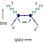
The Example of Electron-Positron Annihilation

In the Feynman diagram above, the properties of the incoming and outgoing particles are measurable.
Their energy or momentum must satisfy Einstein's mass-energy equivalence equation (E² - p² c² = m² c⁴). This interaction allows electrons to exchange their mass and energy, which leads to their annihilation.

The electron e- and the positron e+ have a rest mass of about 0.511 MeV. When these two particles annihilate, their total mass is converted into energy. This energy is released in the form of two photons γ, each with an energy of 0.511 MeV.
The electron and the positron have equal but opposite momentum. When these two particles annihilate, their total momentum is converted into the momentum of the two photons. The photons are emitted in opposite directions, which makes it possible to conserve momentum.
The photons are produced when the electrons disappear.

Main Aspects of Feynman Diagrams

Lines

Lines represent a particle. The color of the line represents the type of particle. For example, blue lines represent electrons, green lines represent photons, red lines represent quarks, etc.

• Solid lines represent fermions (electrons and quarks).
• Wavy lines represent gauge bosons (photons and W/Z bosons) accompanied by their symbol.
• Dotted lines represent exchanges of virtual particles, such as gluon exchanges in interactions between quarks. The Higgs boson is represented by a dotted line accompanied by its symbol.
• Double-arrow lines represent antiparticles (positron, antiproton, etc.), which are the antimatter partners of ordinary particles.
• Wavy lines with bidirectional arrows represent neutral particles (neutron, neutrino, photon) that can interact with positively or negatively charged particles.
• Lines with specific labels represent exotic particles specific to certain theories (axions, tachyons).

Arrows

The arrows in Feynman diagrams do not indicate the direction of time for the particles. They simply indicate the type of particle. However, it is common to represent ordinary particles as moving toward the future, and antiparticles as moving toward the past.

• Fermions are represented by an arrowed line. The arrow points toward the future for ordinary particles and toward the past for antiparticles.
• Antifermions are represented by an arrowed line with an arrow in the opposite direction. The arrow points toward the past for ordinary particles and toward the future for antiparticles.

Vertices

Vertices represent a point in space-time where particles interact. They are represented by connection points where particle lines cross. Vertices are specific locations in a Feynman diagram where particle lines enter or exit.

• For the electromagnetic interaction, involving the exchange of photons, the vertex is generally represented by a point where a particle line (for example, an electron) emits or absorbs a photon. The graphical representation may look like a fork where one line splits into two.
• In the strong interaction between quarks, the vertex is represented by a particle line (quark) emitting or absorbing a gluon. Gluons, the force carriers of the strong interaction, are also represented by lines, and the vertex may look like a fork similar to that of the electromagnetic interaction.
• Weak interactions, such as beta decay, involve the W and Z bosons. The vertices associated with these interactions can be represented by particle lines emitting or absorbing these bosons.

Lines Between Vertices

The lines between vertices represent the propagation of particles through space and time. Each line connecting two vertices corresponds to the trajectory of a specific particle between these two interaction points.

• The line between vertices follows a specific direction, indicating the direction of time in which the particle propagates. In a typical diagram, time progresses from left to right. A particle line from left to right represents a particle propagating toward the future.
• The lines between vertices are drawn so as to respect the conservation laws of charges and other physical quantities. The incoming and outgoing particles in a given process must satisfy these conservation rules.
• In some cases, the lines between vertices may represent the exchange of virtual particles, which are not directly observable but are important for calculating probability amplitudes.

Quantum Numbers

Quantum numbers such as electric charge, flavor, and angular momentum (spin) are represented by particles and their interactions. Quantum numbers are intrinsic characteristics of subatomic particles. They do not change over time and do not depend on the state of a particle. In Feynman diagrams, quantum numbers are represented by specific symbols. Electric charge is represented by a circle, flavor is represented by a letter, and angular momentum is represented by an arrow.

• The electric charge of a particle is often represented by the letter "q". It can be positive, negative, or zero. An electron is represented with a negative charge (-). Positrons, which are the antiparticles of electrons, have a positive charge (+).
• Flavor refers to the type of particle, whether it is a quark of a certain flavor (up, down, strange, charm, top, bottom) or a lepton of a certain generation (electron, muon, tau). The flavor quantum number is often denoted by the letter "f" in the context of particle flavor. For example, for the different types of neutrinos, f = 1, 2, 3 is used for the electron, muon, and tau flavors respectively.
• Angular momentum, also called spin, is often represented by the letter "s" or the symbol "S". Spin is expressed in units of ħ (h bar), the reduced Planck constant. Possible values of spin include 0, 1/2, 1, etc.

Fermions (particles with a spin of 1/2) are generally represented by solid lines. Gauge bosons (particles with a spin of 1) are generally represented by wavy lines. Higgs bosons (particles with a spin of 0) may be represented by special lines in certain diagrams.

• The magnetic quantum number is used to describe the orientation of a particle's angular momentum in a magnetic field. It is often denoted by the letter "m" or "m_s".